42. Job Search I: The McCall Search Model#
“Questioning a McCall worker is like having a conversation with an out-of-work friend: ‘Maybe you are setting your sights too high’, or ‘Why did you quit your old job before you had a new one lined up?’ This is real social science: an attempt to model, to understand, human behavior by visualizing the situation people find themselves in, the options they face and the pros and cons as they themselves see them.” – Robert E. Lucas, Jr.
In addition to what’s in Anaconda, this lecture will need the following libraries:
!pip install quantecon jax
42.1. Overview#
The McCall search model [McCall, 1970] helped transform economists’ way of thinking about labor markets.
To clarify notions such as “involuntary” unemployment, McCall modeled the decision problem of an unemployed worker in terms of factors including
current and likely future wages
impatience
unemployment compensation
To solve the decision problem McCall used dynamic programming.
Here we set up McCall’s model and use dynamic programming to analyze it.
As we’ll see, McCall’s model is not only interesting in its own right but also an excellent vehicle for learning dynamic programming.
Let’s start with some imports:
import matplotlib.pyplot as plt
import numpy as np
import numba
import jax
import jax.numpy as jnp
from typing import NamedTuple
from functools import partial
import quantecon as qe
from quantecon.distributions import BetaBinomial
Matplotlib is building the font cache; this may take a moment.
42.2. The McCall Model#
An unemployed agent receives in each period a job offer at wage \(w_t\).
In this lecture, we adopt the following simple environment:
The offer sequence \(\{w_t\}_{t \geq 0}\) is IID, with \(q(w)\) being the probability of observing wage \(w\) in finite set \(\mathbb{W}\).
The agent observes \(w_t\) at the start of \(t\).
The agent knows that \(\{w_t\}\) is IID with common distribution \(q\) and can use this when computing expectations.
(In later lectures, we will relax these assumptions.)
At time \(t\), our agent has two choices:
Accept the offer and work permanently at constant wage \(w_t\).
Reject the offer, receive unemployment compensation \(c\), and reconsider next period.
The agent is infinitely lived and aims to maximize the expected discounted sum of earnings
The constant \(\beta\) lies in \((0, 1)\) and is called a discount factor.
The smaller is \(\beta\), the more the agent discounts future utility relative to current utility.
The variable \(y_t\) is income, equal to
his/her wage \(w_t\) when employed
unemployment compensation \(c\) when unemployed
42.2.1. A Trade-Off#
The worker faces a trade-off:
Waiting too long for a good offer is costly, since the future is discounted.
Accepting too early is costly, since better offers might arrive in the future.
To decide optimally in the face of this trade-off, we use dynamic programming.
Dynamic programming can be thought of as a two-step procedure that
first assigns values to “states” and
then deduces optimal actions given those values
We’ll go through these steps in turn.
42.2.2. The Value Function#
In order to optimally trade-off current and future rewards, we need to think about two things:
the current payoffs we get from different choices
the different states that those choices will lead to in next period
To weigh these two aspects of the decision problem, we need to assign values to states.
To this end, let \(v^*(w)\) be the total lifetime value accruing to an unemployed worker who enters the current period unemployed when the wage is \(w \in \mathbb{W}\).
(In particular, the agent has wage offer \(w\) in hand and can accept or reject it.)
More precisely, \(v^*(w)\) denotes the value of the objective function (42.1) when an agent in this situation makes optimal decisions now and at all future points in time.
Of course \(v^*(w)\) is not trivial to calculate because we don’t yet know what decisions are optimal and what aren’t!
But think of \(v^*\) as a function that assigns to each possible wage \(s\) the maximal lifetime value that can be obtained with that offer in hand.
A crucial observation is that this function \(v^*\) must satisfy the recursion
for every possible \(w\) in \(\mathbb{W}\).
This is a version of the Bellman equation, which is ubiquitous in economic dynamics and other fields involving planning over time.
The intuition behind it is as follows:
the first term inside the max operation is the lifetime payoff from accepting current offer, since
the second term inside the max operation is the continuation value, which is the lifetime payoff from rejecting the current offer and then behaving optimally in all subsequent periods
If we optimize and pick the best of these two options, we obtain maximal lifetime value from today, given current offer \(w\).
But this is precisely \(v^*(w)\), which is the left-hand side of (42.2).
42.2.3. The Optimal Policy#
Suppose for now that we are able to solve (42.2) for the unknown function \(v^*\).
Once we have this function in hand we can behave optimally (i.e., make the right choice between accept and reject).
All we have to do is select the maximal choice on the right-hand side of (42.2).
The optimal action is best thought of as a policy, which is, in general, a map from states to actions.
Given any \(w\), we can read off the corresponding best choice (accept or reject) by picking the max on the right-hand side of (42.2).
Thus, we have a map from \(\mathbb W\) to \(\{0, 1\}\), with 1 meaning accept and 0 meaning reject.
We can write the policy as follows
Here \(\mathbf{1}\{ P \} = 1\) if statement \(P\) is true and equals 0 otherwise.
We can also write this as
where
Here \(\bar w\) (called the reservation wage) is a constant depending on \(\beta, c\) and the wage distribution.
The agent should accept if and only if the current wage offer exceeds the reservation wage.
In view of (42.3), we can compute this reservation wage if we can compute the value function.
42.3. Computing the Optimal Policy: Take 1#
To put the above ideas into action, we need to compute the value function at each \(w \in \mathbb W\).
To simplify notation, let’s set
The value function is then represented by the vector \(v^* = (v^*(i))_{i=1}^n\).
In view of (42.2), this vector satisfies the nonlinear system of equations
42.3.1. The Algorithm#
To compute this vector, we use successive approximations:
Step 1: pick an arbitrary initial guess \(v \in \mathbb R^n\).
Step 2: compute a new vector \(v' \in \mathbb R^n\) via
Step 3: calculate a measure of a discrepancy between \(v\) and \(v'\), such as \(\max_i |v(i)- v'(i)|\).
Step 4: if the deviation is larger than some fixed tolerance, set \(v = v'\) and go to step 2, else continue.
Step 5: return \(v\).
For a small tolerance, the returned function \(v\) is a close approximation to the value function \(v^*\).
The theory below elaborates on this point.
42.3.2. Fixed Point Theory#
What’s the mathematics behind these ideas?
First, one defines a mapping \(T\) from \(\mathbb R^n\) to itself via
(A new vector \(Tv\) is obtained from given vector \(v\) by evaluating the r.h.s. at each \(i\).)
The element \(v_k\) in the sequence \(\{v_k\}\) of successive approximations corresponds to \(T^k v\).
This is \(T\) applied \(k\) times, starting at the initial guess \(v\)
One can show that the conditions of the Banach fixed point theorem are satisfied by \(T\) on \(\mathbb R^n\).
One implication is that \(T\) has a unique fixed point in \(\mathbb R^n\).
That is, a unique vector \(\bar v\) such that \(T \bar v = \bar v\).
Moreover, it’s immediate from the definition of \(T\) that this fixed point is \(v^*\).
A second implication of the Banach contraction mapping theorem is that \(\{ T^k v \}\) converges to the fixed point \(v^*\) regardless of \(v\).
42.3.3. Implementation#
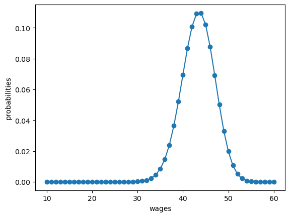
Our default for \(q\), the distribution of the state process, will be Beta-binomial.
n, a, b = 50, 200, 100                        # default parameters
q_default = jnp.array(BetaBinomial(n, a, b).pdf())
Our default set of values for wages will be
w_min, w_max = 10, 60
w_default = jnp.linspace(w_min, w_max, n+1)
Here’s a plot of the probabilities of different wage outcomes:
fig, ax = plt.subplots()
ax.plot(w_default, q_default, '-o', label='$q(w(i))$')
ax.set_xlabel('wages')
ax.set_ylabel('probabilities')

plt.show()
We will use JAX to write our code.
We’ll use NamedTuple for our model class to maintain immutability, which works well with JAX’s functional programming paradigm.
Here’s a class that stores the model parameters with default values.
class McCallModel(NamedTuple):
    c: float = 25               # unemployment compensation
    β: float = 0.99             # discount factor
    w: jnp.ndarray = w_default  # array of wage values, w[i] = wage at state i
    q: jnp.ndarray = q_default  # array of probabilities
We implement the Bellman operator \(T\) from (42.6) as follows
def T(model: McCallModel, v: jnp.ndarray):
    c, β, w, q = model
    accept = w / (1 - β)
    reject = c + β * v @ q
    return jnp.maximum(accept, reject)
Based on these defaults, let’s try plotting the first few approximate value functions in the sequence \(\{ T^k v \}\).
We will start from guess \(v\) given by \(v(i) = w(i) / (1 - β)\), which is the value of accepting at every given wage.
model = McCallModel()
c, β, w, q = model
v = w / (1 - β)   # Initial condition
fig, ax = plt.subplots()

num_plots = 6
for i in range(num_plots):
    ax.plot(w, v, '-', alpha=0.6, lw=2, label=f"iterate {i}")
    v = T(model, v)

ax.legend(loc='lower right')
ax.set_xlabel('wage')
ax.set_ylabel('value')
plt.show()
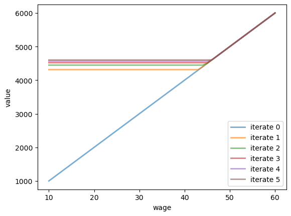
You can see that convergence is occurring: successive iterates are getting closer together.
Here’s a more serious iteration effort to compute the limit, which continues until measured deviation between successive iterates is below tol.
Once we obtain a good approximation to the limit, we will use it to calculate the reservation wage.
def compute_reservation_wage(
        model: McCallModel,   # instance containing default parameters
        v_init: jnp.ndarray,  # initial condition for iteration
        tol: float=1e-6,      # error tolerance
        max_iter: int=500,    # maximum number of iterations for loop
    ):
    "Computes the reservation wage in the McCall job search model."
    c, β, w, q = model
    i = 0
    error = tol + 1
    v = v_init

    while i < max_iter and error > tol:
        v_next = T(model, v)
        error = jnp.max(jnp.abs(v_next - v))
        v = v_next
        i += 1

    res_wage = (1 - β) * (c + β * v @ q)
    return v, res_wage
The cell computes the reservation wage at the default parameters
model = McCallModel()
c, β, w, q = model
v_init = w / (1 - β)  # initial guess
v, res_wage = compute_reservation_wage(model, v_init)
print(res_wage)
47.316475
42.3.4. Comparative Statics#
Now that we know how to compute the reservation wage, let’s see how it varies with parameters.
In particular, let’s look at what happens when we change \(\beta\) and \(c\).
As a first step, given that we’ll use it many times, let’s create a more efficient, jit-complied version of the function that computes the reservation wage:
@jax.jit
def compute_res_wage_jitted(
        model: McCallModel,   # instance containing default parameters
        v_init: jnp.ndarray,  # initial condition for iteration
        tol: float=1e-6,      # error tolerance
        max_iter: int=500,    # maximum number of iterations for loop
    ):
    c, β, w, q = model
    i = 0
    error = tol + 1
    initial_state = v_init, i, error

    def cond(loop_state):
        v, i, error = loop_state
        return jnp.logical_and(i < max_iter, error > tol)

    def update(loop_state):
        v, i, error = loop_state
        v_next = T(model, v)
        error = jnp.max(jnp.abs(v_next - v))
        i += 1
        new_loop_state = v_next, i, error
        return new_loop_state

    final_state = jax.lax.while_loop(cond, update, initial_state)
    v, i, error = final_state

    res_wage = (1 - β) * (c + β * v @ q)
    return v, res_wage
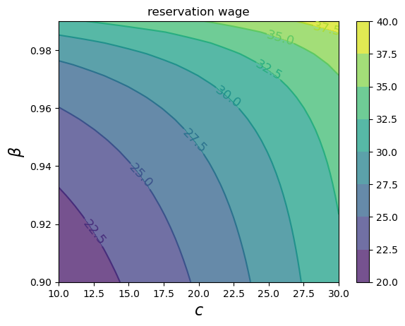
Now we compute the reservation wage at each \(c, \beta\) pair.
grid_size = 25
c_vals = jnp.linspace(10.0, 30.0, grid_size)
β_vals = jnp.linspace(0.9, 0.99, grid_size)

res_wage_matrix = np.empty((grid_size, grid_size))
model = McCallModel()
v_init = model.w / (1 - model.β)

for i, c in enumerate(c_vals):
    for j, β in enumerate(β_vals):
        model = McCallModel(c=c, β=β)
        v, res_wage = compute_res_wage_jitted(model, v_init)
        v_init = v
        res_wage_matrix[i, j] = res_wage

fig, ax = plt.subplots()
cs1 = ax.contourf(c_vals, β_vals, res_wage_matrix.T, alpha=0.75)
ctr1 = ax.contour(c_vals, β_vals, res_wage_matrix.T)
plt.clabel(ctr1, inline=1, fontsize=13)
plt.colorbar(cs1, ax=ax)
ax.set_title("reservation wage")
ax.set_xlabel("$c$", fontsize=16)
ax.set_ylabel("$β$", fontsize=16)
ax.ticklabel_format(useOffset=False)
plt.show()
As expected, the reservation wage increases with both patience and unemployment compensation.
42.4. Computing an Optimal Policy: Take 2#
The approach to dynamic programming just described is standard and broadly applicable.
But for our McCall search model there’s also an easier way that circumvents the need to compute the value function.
Let \(h\) denote the continuation value:
The Bellman equation can now be written as
Substituting this last equation into (42.7) gives
This is a nonlinear equation that we can solve for \(h\).
As before, we will use successive approximations:
Step 1: pick an initial guess \(h\).
Step 2: compute the update \(h'\) via
Step 3: calculate the deviation \(|h - h'|\).
Step 4: if the deviation is larger than some fixed tolerance, set \(h = h'\) and go to step 2, else return \(h\).
One can again use the Banach contraction mapping theorem to show that this process always converges.
The big difference here, however, is that we’re iterating on a scalar \(h\), rather than an \(n\)-vector, \(v(i), i = 1, \ldots, n\).
Here’s an implementation:
@jax.jit
def compute_reservation_wage_two(
        model: McCallModel,   # instance containing default parameters
        tol: float=1e-5,      # error tolerance
        max_iter: int=500,    # maximum number of iterations for loop
    ):
    c, β, w, q = model
    h = (w @ q) / (1 - β)  # initial condition
    i = 0
    error = tol + 1
    initial_loop_state = i, h, error

    def cond(loop_state):
        i, h, error = loop_state
        return jnp.logical_and(i < max_iter, error > tol)

    def update(loop_state):
        i, h, error = loop_state
        s = jnp.maximum(w / (1 - β), h)
        h_next = c + β * (s @ q)
        error = jnp.abs(h_next - h)
        i_next = i + 1
        new_loop_state = i_next, h_next, error
        return new_loop_state

    final_state = jax.lax.while_loop(cond, update, initial_loop_state)
    i, h, error = final_state

    # Compute and return the reservation wage
    return (1 - β) * h
You can use this code to solve the exercise below.
42.5. Exercises#
Exercise 42.1
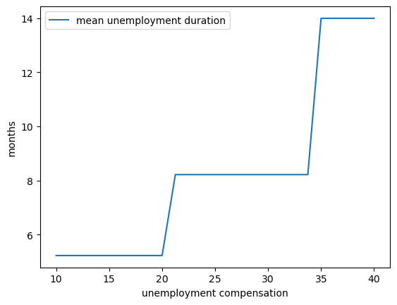
Compute the average duration of unemployment when \(\beta=0.99\) and \(c\) takes the following values
c_vals = np.linspace(10, 40, 25)
That is, start the agent off as unemployed, compute their reservation wage given the parameters, and then simulate to see how long it takes to accept.
Repeat a large number of times and take the average.
Plot mean unemployment duration as a function of \(c\) in c_vals.
Solution to Exercise 42.1
Here’s a solution using Numba.
# Convert JAX arrays to NumPy arrays for use with Numba
q_default_np = np.array(q_default)
w_default_np = np.array(w_default)
cdf = np.cumsum(q_default_np)

@numba.jit
def compute_stopping_time(w_bar, seed=1234):
    """
    Compute stopping time by drawing wages until one exceeds w_bar.
    """
    np.random.seed(seed)
    t = 1
    while True:
        # Generate a wage draw
        w = w_default_np[qe.random.draw(cdf)]

        # Stop when the draw is above the reservation wage
        if w >= w_bar:
            stopping_time = t
            break
        else:
            t += 1
    return stopping_time

@numba.jit(parallel=True)
def compute_mean_stopping_time(w_bar, num_reps=100000):
    """
    Generate a mean stopping time over `num_reps` repetitions by
    drawing from `compute_stopping_time`.
    """
    obs = np.empty(num_reps)
    for i in numba.prange(num_reps):
        obs[i] = compute_stopping_time(w_bar, seed=i)
    return obs.mean()

c_vals = np.linspace(10, 40, 25)
stop_times = np.empty_like(c_vals)
for i, c in enumerate(c_vals):
    mcm = McCallModel(c=c)
    w_bar = compute_reservation_wage_two(mcm)
    stop_times[i] = compute_mean_stopping_time(float(w_bar))

fig, ax = plt.subplots()

ax.plot(c_vals, stop_times, label="mean unemployment duration")
ax.set(xlabel="unemployment compensation", ylabel="months")
ax.legend()

plt.show()
And here’s a solution using JAX.
cdf = jnp.cumsum(q_default)

@jax.jit
def compute_stopping_time(w_bar, key):
    """
    Compute stopping time by drawing wages until one exceeds `w_bar`.
    """
    def update(loop_state):
        t, key, accept = loop_state
        key, subkey = jax.random.split(key)
        u = jax.random.uniform(subkey)
        w = w_default[jnp.searchsorted(cdf, u)]
        accept = w >= w_bar
        t = t + 1
        return t, key, accept

    def cond(loop_state):
        _, _, accept = loop_state
        return jnp.logical_not(accept)

    initial_loop_state = (0, key, False)
    t_final, _, _ = jax.lax.while_loop(cond, update, initial_loop_state)
    return t_final


@partial(jax.jit, static_argnames=('num_reps',))
def compute_mean_stopping_time(w_bar, num_reps=100000, seed=1234):
    """
    Generate a mean stopping time over `num_reps` repetitions by
    drawing from `compute_stopping_time`.
    """
    # Generate a key for each MC replication
    key = jax.random.PRNGKey(seed)
    keys = jax.random.split(key, num_reps)

    # Vectorize compute_stopping_time and evaluate across keys
    compute_fn = jax.vmap(compute_stopping_time, in_axes=(None, 0))
    obs = compute_fn(w_bar, keys)

    # Return mean stopping time
    return jnp.mean(obs)

c_vals = jnp.linspace(10, 40, 25)

def compute_stop_time_for_c(c):
    """Compute mean stopping time for a given compensation value c."""
    model = McCallModel(c=c)
    w_bar = compute_reservation_wage_two(model)
    return compute_mean_stopping_time(w_bar)

# Vectorize across all c values
stop_times = jax.vmap(compute_stop_time_for_c)(c_vals)

fig, ax = plt.subplots()

ax.plot(c_vals, stop_times, label="mean unemployment duration")
ax.set(xlabel="unemployment compensation", ylabel="months")
ax.legend()

plt.show()

At least for our hardware, Numba is faster on the CPU while JAX is faster on the GPU.
Exercise 42.2
The purpose of this exercise is to show how to replace the discrete wage offer distribution used above with a continuous distribution.
This is a significant topic because many convenient distributions are continuous (i.e., have a density).
Fortunately, the theory changes little in our simple model.
Recall that \(h\) in (42.7) denotes the value of not accepting a job in this period but then behaving optimally in all subsequent periods:
To shift to a continuous offer distribution, we can replace (42.7) by
Equation (42.8) becomes
The aim is to solve this nonlinear equation by iteration, and from it obtain the reservation wage.
Try to carry this out, setting
the state sequence \(\{ s_t \}\) to be IID and standard normal and
the wage function to be \(w(s) = \exp(\mu + \sigma s)\).
You will need to implement a new version of the McCallModel class that
assumes a lognormal wage distribution.
Calculate the integral by Monte Carlo, by averaging over a large number of wage draws.
For default parameters, use c=25, β=0.99, σ=0.5, μ=2.5.
Once your code is working, investigate how the reservation wage changes with \(c\) and \(\beta\).
Solution to Exercise 42.2
Here is one solution:
class McCallModelContinuous(NamedTuple):
    c: float              # unemployment compensation
    β: float              # discount factor
    σ: float              # scale parameter in lognormal distribution
    μ: float              # location parameter in lognormal distribution
    w_draws: jnp.ndarray  # draws of wages for Monte Carlo


def create_mccall_continuous(
        c=25, β=0.99, σ=0.5, μ=2.5, mc_size=1000, seed=1234
    ):
    key = jax.random.PRNGKey(seed)
    s = jax.random.normal(key, (mc_size,))
    w_draws = jnp.exp(μ + σ * s)
    return McCallModelContinuous(c=c, β=β, σ=σ, μ=μ, w_draws=w_draws)


@jax.jit
def compute_reservation_wage_continuous(model, max_iter=500, tol=1e-5):
    c, β, σ, μ, w_draws = model.c, model.β, model.σ, model.μ, model.w_draws

    h = jnp.mean(w_draws) / (1 - β)  # initial guess

    def update(state):
        h, i, error = state
        integral = jnp.mean(jnp.maximum(w_draws / (1 - β), h))
        h_next = c + β * integral
        error = jnp.abs(h_next - h)
        return h_next, i + 1, error

    def cond(state):
        h, i, error = state
        return jnp.logical_and(i < max_iter, error > tol)

    initial_state = (h, 0, tol + 1)
    h_final, _, _ = jax.lax.while_loop(cond, update, initial_state)

    # Now compute the reservation wage
    return (1 - β) * h_final
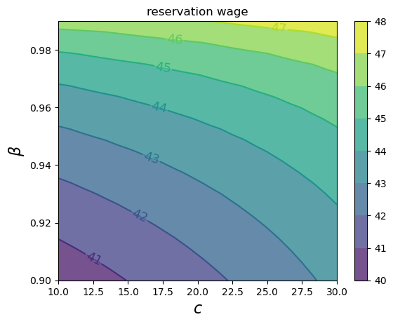
Now we investigate how the reservation wage changes with \(c\) and \(\beta\).
We will do this using a contour plot.
grid_size = 25
c_vals = jnp.linspace(10.0, 30.0, grid_size)
β_vals = jnp.linspace(0.9, 0.99, grid_size)

def compute_R_element(c, β):
    model = create_mccall_continuous(c=c, β=β)
    return compute_reservation_wage_continuous(model)

# Create meshgrid and vectorize computation
c_grid, β_grid = jnp.meshgrid(c_vals, β_vals, indexing='ij')
compute_R_vectorized = jax.vmap(
    jax.vmap(compute_R_element,
    in_axes=(None, 0)),
    in_axes=(0, None))
R = compute_R_vectorized(c_vals, β_vals)
fig, ax = plt.subplots()

cs1 = ax.contourf(c_vals, β_vals, R.T, alpha=0.75)
ctr1 = ax.contour(c_vals, β_vals, R.T)

plt.clabel(ctr1, inline=1, fontsize=13)
plt.colorbar(cs1, ax=ax)


ax.set_title("reservation wage")
ax.set_xlabel("$c$", fontsize=16)
ax.set_ylabel("$β$", fontsize=16)

ax.ticklabel_format(useOffset=False)

plt.show()